You can count the number of occurrences of anything, using criteria for either numbers or text in the range of cells. In this article, you’ll learn the syntax of the COUNTIF function, as well as a few examples.
COUNTIF Syntax in Google Sheets
First, let’s look at how you need to structure the COUNTIF function in order for it to work right. There are only two parameters to use: COUNTIF(range, criterion) These parameters identify the range to search through, and the conditions you want to use to count.
range: A range of columns and rows that include all of the data you want to search through.criterion: The test you want to apply to the range to find matching conditions.
The criterion you can use for numerical data include operators like =, >, >=, <, <=, or <>. You can also just type a specific number to get an exact match. If the data you’re searching through is text, you can either type the exact text you want to find or include wildcards. Text wildcards include:
? – Let’s you search for a word that includes any character where you’ve placed the ? punctuation.* – Match contiguous characters before, after, or between the wildcard character.
Now that you understand the parameters, let’s take a look at how the COUNTIF function searches through a range.
Using COUNTIF on Ranges
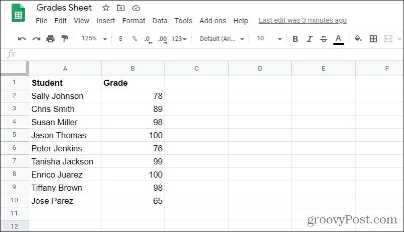
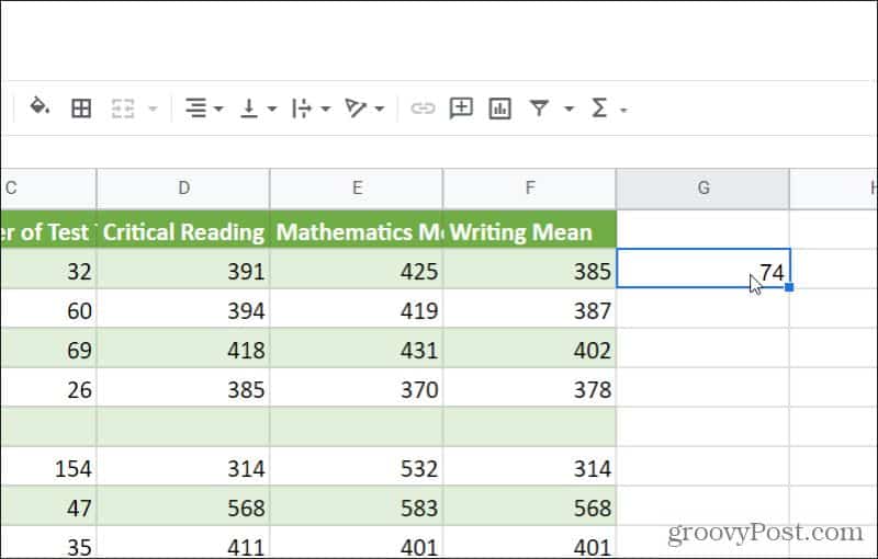
Consider a scenario where you have a small range of cells containing a list of student names and their grades on a test.
In this case, the range you’ll want to use in the COUNTIF function is A2:B10. If you want to find all grades over 80, the COUNTIF function will look like this: =COUNTIF(A1:B10, “>80”) If you type this into one of the blank cells and press the Enter key, COUNTIF performs the search as follows: Keep in mind when using this function that if both rows have numbers, in a case like this the tally will include numbers in either column. So craft your criterion parameter carefully.
Example 1: Numeric Limits
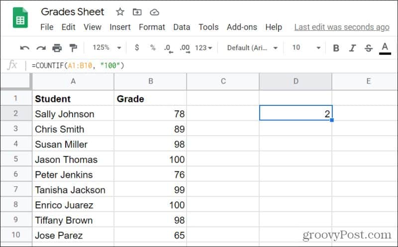
The example above was one method of counting items in a range when the data is numeric. The example above is one using comparison operators. You can also search for an exact number. For example, if you type =COUNTIF(A1:B10, “100”) and press Enter, you’ll see a list of how many 100s were on the list.
In this case, there are two. You could also get a count of all numbers that aren’t equal to 100 by typing =COUNTIF(A1:B10, “<>100”)
In this case, the result is 18, because 18 of the numbers are not 100. As you can see, using COUNTIF with numeric data is easy!
Example 2: Counting Specific Records
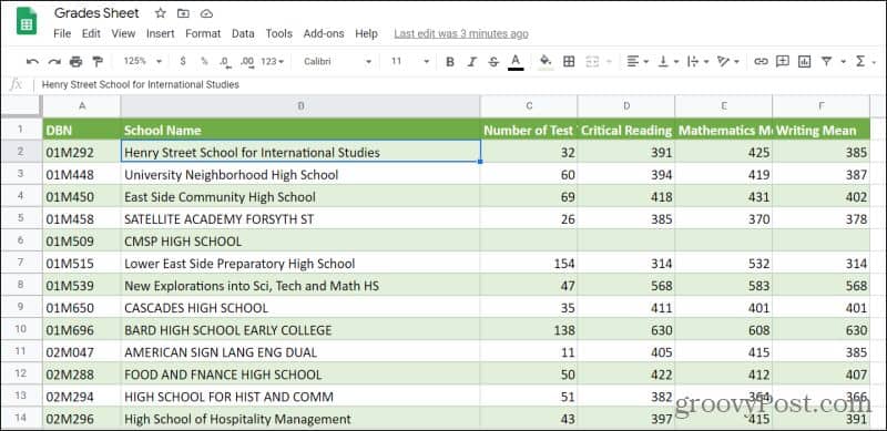
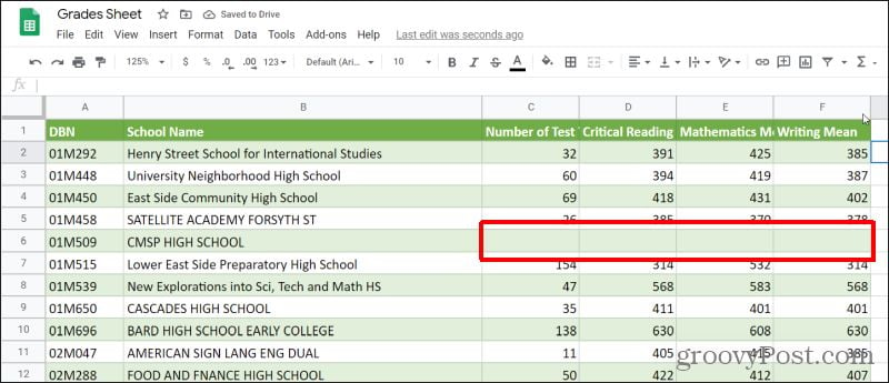
If you’re working with text data, then comparison operators won’t work. In these cases, you’ll want to type in the exact text you’re searching for. COUNTIF will tell you how many times that exact text occurred. This is helpful when you’re looking for specific records in a list of data. The example below is a list of schools and their national SAT scores.
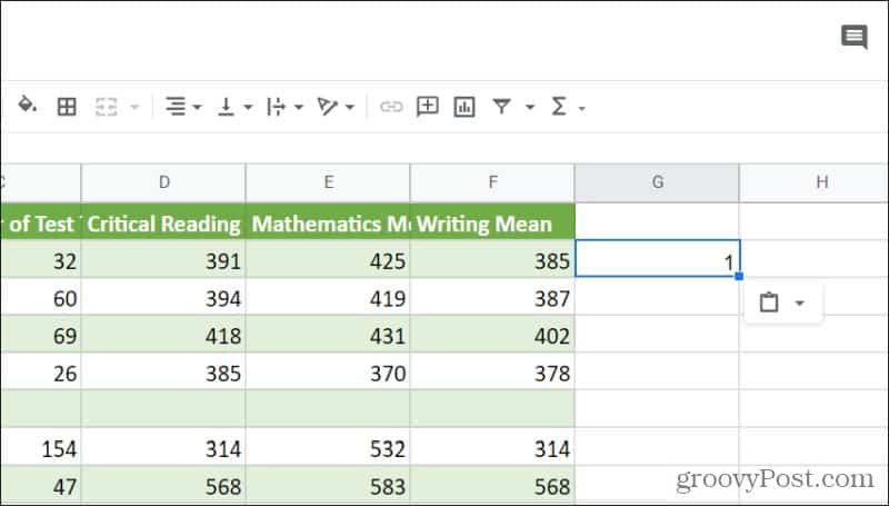
There’s no way of knowing how many times a school shows up without searching down the School Name column manually. Instead, you can use the COUNTIF function to search for the number of times a specific school shows up. To do this, you would type: =COUNTIF(A1:B10, “pace high school”). When you press Enter, you’ll see the result is 1.
This means “pace high school” only shows up in the list of schools once. You can also use special characters to look for partial records. For example, if you type =COUNTIF(A1:B10, “college”), you’ll see the number of records that contain the word “college”.
In this case, that’s 14 cases where the school name contains “college”. As an alternative, you could also use the “?” character to look for schools that contain the words “of” or “if” by typing: =COUNTIF(A1:B10, “?f”). Note: The search text you use isn’t case sensitive, so you can use upper case or lower case letters, and it will still find the right results.
Example 3: Filtering Out Blanks
There are two ways to handle blanks using the COUNTIF function. You can either count blank cells or count non-blank cells. Keep in mind that if you’re searching an entire range, the COUNTIF function will count every blank cell.
However, if you’re only interested in the number of rows that have blank cells, you should make the range a single row instead. So, in this case, you would type: =COUNTIF(C1:C460, “”). This focuses your search on one column, and returns all the blanks.
You could also search for the number of rows that aren’t blank. To do this, type the following: =COUNTIF(C1:C460, “<>”). Press Enter and you’ll see the number of non-blank cells in the column.
Above are examples of all of the parameters you can use with the COUNTIF function. If you’re interested in exploring how to search ranges using multiple criteria, you could also explore using the COUNTIF function. You could also explore doing similar things with functions in Excel if you prefer.


![]()
